Christopher Kang, CS @ UW + Technical Intern @ PNNL

Foreword

Molecular simulation has been described as “Quantum’s killer app”. The hope is, with quantum algorithms and a bit of math, we can understand the hidden lives of molecules.

Andrew’s intro to the core concepts of Hamiltonian simulation was fantastic, and I wanted to provide an add-on that discusses more in-depth material on the theoretical chemistry foundations, quantum circuits, and open problems.

Table of Contents

• Context
• Fermionic Hamiltonian and Fermionic Operators
• The Jordan-Wigner Transform
• Circuits
• Analysis, Alternatives, and Next Steps

Context

Motivation

As a primary question: why do we care about molecular simulation?

The first reason is basic research: even today, we cannot predict the precise structure of molecules or proteins. Understanding these molecules could tell us more about our universe - and how its smallest building blocks look.

The second reason is real-world applicability: large-scale simulations could fundamentally transform chemical design. One example is in drug discovery: suppose you have multiple candidates for a vaccine (say, for a global pandemic). Which candidate do you send to phased clinical trials? With a sufficiently large molecular simulation, you could screen potential therapeutics digitally (instead of through assays / human testing), which would be cheaper, quicker, and safer. 

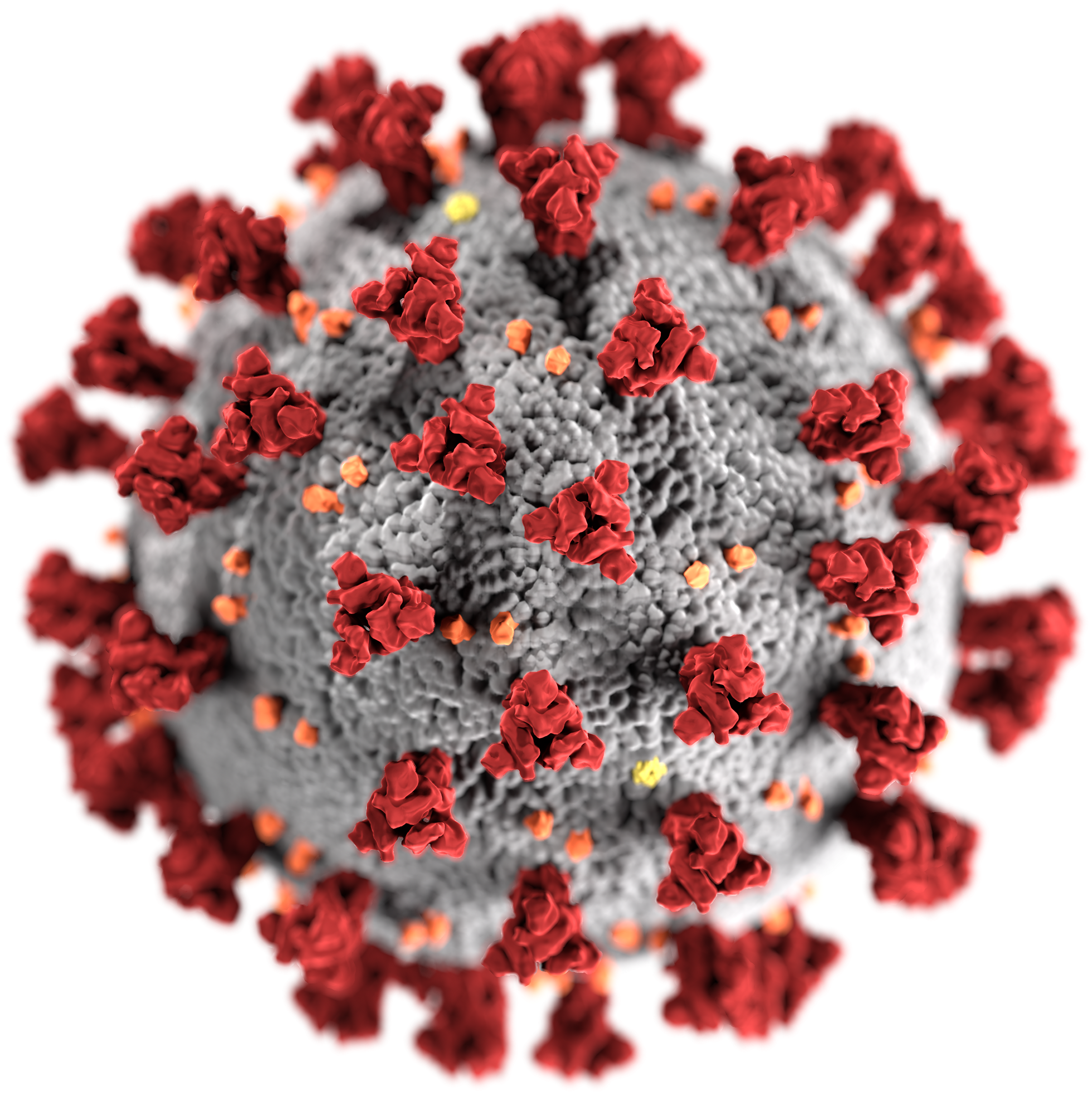Source: CDC / Wikimedia Commons

Our overall goal with this algorithm is to identify the superposition of electrons in a molecule and the configuration’s energy level. By testing different configurations, we’ll be able to find the ground state configuration (and thus the “normal” state of the molecule).

Algorithm Strategy

1. In the first section, we’ll outline the fundamental problem: simulating a Hamiltonian and identifying its eigenvalue.
2. Then, using the Jordan-Wigner transform, we can map the Hamiltonian to a quantum computer’s native architecture.
3. Next, we’ll identify the specific circuits that can be used.
4. Finally, we’ll identify limitations with the strategy and optimizations that could be applied.

Fermionic Hamiltonian and Fermionic Operators

Key Ideas

The Hamiltonian is a matrix describing the dynamics of fermions (e.g. electrons). By identifying eigenvectors of the Hamiltonian, we can find stable electron configurations. If we identify the eigenvector with the lowest eigenvalue, we have identified the ground configuration of the molecule.

Operators

The fermionic operators come in two forms: annihilation $a$ and creation $a^{\dagger}$. The annihilation operator, well, annihilates electrons! (Similarly, the creation operator creates them). The operators take the following form:

\[a_p = \bigotimes_{k = 0}^{p - 1} Z_k \otimes \begin{bmatrix} 0 & 1 \\ 0 & 0 \end{bmatrix}, a^{\dagger}_p = \bigotimes_{k = 0}^{p - 1} Z_k \otimes \begin{bmatrix} 0 & 0 \\ 1 & 0 \end{bmatrix}\]

This looks complicated, but let’s begin by looking at the matrices. Note that:

\[\begin{bmatrix} 0 & 1 \\ 0 & 0 \end{bmatrix} | 1 \rangle = |0\rangle, \begin{bmatrix} 0 & 0 \\ 1 & 0 \end{bmatrix} | 0 \rangle = |1 \rangle\]

In essence, the left matrix “annihilates” an electron and the right matrix “creates” an electron (exactly as we desired!) But, what do the $\otimes_{k = 0}^{p - 1} Z_k$ mean? These are actually artifacts from the definition of fermionic operators which require anticommutation relations (basically, we want $a^\dagger_p a^\dagger_q = - a^\dagger_q a^\dagger_p$, etc).

So, we can create/delete electrons. How do we understand the dynamics of electrons and orbitals?

Hamiltonian

The Hamiltonian ($H$) describes the dynamics of the electrons - quantum mechanics has structured the problem like a differential equation. We want to find a solution $|\psi(t)\rangle$ that explains the modeling from the dif-eq:

\[-i \hbar\frac{d}{d t} |\psi(t)\rangle = H |\psi(t) \rangle\]

Where $\vert \psi(t) \rangle$ is the “state vector” or configuration of the electrons with respect to time $t$, and the Hamiltonian is:

\[H = \sum_{p, q} h_{pq} a^{\dagger}_p a_q + \sum_{p, q, r, s} h_{pqrs} a^{\dagger}_p a^{\dagger}_q a_r a_s\]

These two sums comprise the Hamiltonian - the left sum is the “one-body terms” (moving an electron from \(q\) to \(p\)) and the right sum is the “two-body terms” (moving electrons from \(r, s\) to \(p, q\)).

It turns out \(H\) is actually hermitian (by symmetry). So, \(-iHt\) is also anti-hermitian when \(t\) real, so \(e^{-iHt}\) unitary (this is a given property). So, we just need to find a circuit that will actually apply \(e^{-iHt}\), which evolves our initial \(\vert \psi (0) \rangle\) state into \(\vert \psi (t) \rangle\).

Additionally, if we are given an eigenvector $\vert \psi_v\rangle$ of $H$, then the eigenvalue \(\lambda_v\) is the associated energy level. So, this yields two key problems: implementing the \(e^{-iHt}\) simulation and the eigenvalue \(\lambda_v\).

The Jordan-Wigner Transform

Key Ideas

The Jordan-Wigner (JW) transform is fascinating because it maps our fermionic Hamiltonian \(H\) into the sum of Pauli operators, meaning that \(e^{-iHt}\) is actually implementable in terms of our existing Paulis.

Using the Transform

While we have the Hamiltonian, the fermionic operators that comprise it are foreign to quantum devices. We want to transform $H$ into Paulis, something that we can implement. Looking at the matrix form, we see:

\[\begin{bmatrix} 0 & 1 \\ 0 & 0 \end{bmatrix} = \frac{X + iY}{2}, \begin{bmatrix} 0 & 0 \\ 1 & 0 \end{bmatrix} = \frac{X - iY}{2}\]

Now, to account for the anticommutation relations, we add a series of $Z$ gates to the end of the operator, yielding a final translation of: \(a^{\dagger}_p = \Big( \bigotimes_{k = 0}^{p - 1} Z_k \Big) \otimes \Big(\frac{X_p - iY_p}{2} \Big), a_p = \Big( \bigotimes_{k = 0}^{p - 1} Z_k \Big) \otimes \Big( \frac{X_p + iY_p}{2} \Big)\)

This is tremendous! Even though $a^{\dagger}_p, a_q$ may not be unitary, they are Hermitian; so, if we make them anti-Hermitian and exponentiate, they will be unitary! Note that our original Hamiltonian can be translated, eventually yielding:

\[H = \sum c_k H_k\]

Where $c_k$ is a real coefficient and $H_k$ is a Hamiltonian that is the sum of Paulis. This means that, when exponentiated,

\[e^{-i \sum c_k H_k t} \approx \prod_{k} e^{-i c_k H_k t}\]

Essentially, we just need to implement a series of sub-Hamiltonians $e^{-i c_k H_k t}$, whose unitaries product yields the desired evolution.

Circuits

Implementing the Hamiltonians

Each of the terms from $\sum h_{pq} a^\dagger_p a_q$, $\sum h_{pqrs} a^\dagger_p a^\dagger_q a_r a_s$ has a direct circuit analogue (see Table A1 of Whitfield et al.). We can segment the terms into the following classes*:

• $a^\dagger_p a_p$ (PP)
• $a^\dagger_p a_q + a^\dagger_q a_p$ (PQ)
• $a^\dagger_p a^\dagger_q a_q a_p$ (PQQP)
• $a^\dagger_p a^\dagger_q a_q a_r + a^\dagger_r a^\dagger_q a_q a_p$ (PQQR)
• $a^\dagger_p a^\dagger_q a_r a_s + a^\dagger_s a^\dagger_r a_q a_p$ (PQRS)

*Some of these terms have their conjugates by symmetry of electron operations.

For simplicity, we will only solve for the simplest term (PP), but all have explicit Pauli formulations that can be found algebraically. Note that: \(a^\dagger_p a_p = \bigotimes_{k = 0}^{p - 1} Z_k \otimes \Big(\frac{X_p - iY_p}{2} \Big) \bigotimes_{k = 0}^{p - 1} Z_k \otimes \Big(\frac{X_p + iY_p}{2} \Big) \\ = \frac{X_p X_p - iY_p X_p + iX_p Y_p + Y_p Y_p}{4} \\ = \frac{\mathbb{1} - Z_p}{2}\)

Where $\mathbb{1}$ is the identity matrix. So, $e^{-i(\mathbb{1} - Z_p)t / 2} \approx e^{-it/2} e^{iZ_pt/2}$, where the first is implementable trivially by global phase and the second is implementable as Rz. Thus, the PP term is implementable.

Estimating Eigenvalues

Now, suppose we continue the logic above and have found an approximation for $e^{-iHt}$ in terms of $\prod_k e^{-i c_k H_k t}$. How could we identify the eigenvalue $\lambda_v$? We know by supposition that $H |\psi_v\rangle = \lambda_v |\psi_v \rangle$. Then, does $e^{-iHt} |\psi_v \rangle$ have a clear form?

Via the Taylor series expansion, we know: \(e^{-iHt} = \sum_{k = 0}^\infty \frac{(-iHt)^k}{k!} |\psi_v \rangle \\ = \sum_{k = 0}^\infty \frac{(-it)^k}{k!} H^k |\psi_v \rangle \\ = \sum_{k = 0}^\infty \frac{(-it)^k}{k!} \lambda_v^k |\psi_v \rangle \\ = \sum_{k = 0}^\infty \frac{(-i\lambda_v t)^k}{k!} |\psi_v \rangle \\ = e^{-i \lambda_v t} |\psi_v \rangle\)

So, the eigenvalue actually emerges in the phase applied! Thus, we apply quantum phase estimation (QPE) on the Hamiltonian to identify $e^{-i\lambda_v t}$, and by proxy, $\lambda_v$.

Analysis, Alternatives, and Next Steps

Advantages

In this section, we’ll note some of the advantages of the phase estimation-based (PE) simulation algorithm.

Polynomial scaling Each Hamiltonian term simulated only takes, at most, linear time. So, overall, the simulation is still polynomial with both time and space complexity in number of Hamiltonian terms.

In addition, space complexity is linear with the number of orbitals, as each qubit corresponds directly to an orbital. This means that, for each additional error corrected qubit, the molecule size can increase by an orbital (far better than the exponential scaling of classical algorithms).

Simple implementation The PE algorithm natively uses operations which will likely be common on quantum devices - namely, QPE and simple rotation/CNOT gates.

Ansatz Preparation While not discussed, preparing $\vert \psi\rangle$ on a quantum computer is actually much more straightforward than on a classical computer. Parametrized methods like Unitary Coupled Cluster (UCC) can be directly implemented on quantum comptuers with techniques similar to the ones used for simulation.

Challenges

Circuit depth Even though the simulation only has a polynomial number of gates, they often require entire sections of qubits to be engaged in computation, greatly increasing circuit depth. This means that PE simulation is unobtainable on NISQ devices.

Precision required Chemical accuracy is within 0.0016 Hartrees of the actual result of a molecule. This is an incredibly small number, requiring at least 13 qubits reserved for QPE. Even slight deviations during implementation can affect this value, meaning that high fidelity devices are needed to accurately simulate molecules.

Next Steps

This was a summative review of PE based simulation, but there are some next steps for those who are curious!

For more on the error scaling of $e^{-iHt} - \prod_k e^{-i c_k H_k t}$, you should look at the Lie-Trotter-Suzuki product formulas used to derive the error bounds.

For more on optimizing Trotterization, Earl Campbell wrote a short paper on Randomized Hamiltonian Compilation that modifies the Trotter circuits stochastically to reduce depth while maintaining comparable error bounds (I’ve also written a summary).

Last, if you’re interested in alternative methods for simulation, the Variational Quantum Eigensolver (VQE) is known for its near-term applicability and ease of implementation.

Thanks + Works Referenced

I hope you enjoyed this more technical overview! The marriage of theoretical chemistry, algorithm design, and real-world constraints really makes simulation an exciting problem for quantum computers.

I learned most of this material through James Whitfield’s paper, which I’ve compiled into slides prepared for the quantum course at UW that I TA’d. If you have further questions, please reach out! Happy to chat :)